
很多小伙伴不知道Microsoft Excel怎么设置误差线,所以下面小编就分享了Microsoft Excel设置误差线的方法,一起跟着小编来看看吧,相信对大家会有帮助。
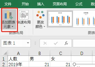
1、首先我们可以在图表中找到“添加图标元素”的按键,如下图所示。
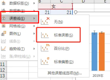
2、然后在“误差线”中找到“标准误差”,如下图所示。
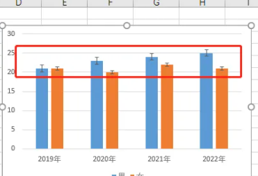
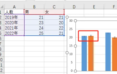
3、随后就可以看到误差线了,如下图所示。
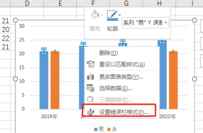
4、我们也可以右键设置错误格式,如下图所示。
5、最后就可以根据美观程度做出更改,如下图所示。
上面就是小编为大家带来的Microsoft Excel怎么设置误差线的全部内容,希望对大家能够有所帮助哦。
 超凡先锋
超凡先锋 途游五子棋
途游五子棋 超级玛丽
超级玛丽 口袋妖怪绿宝石
 地牢求生
地牢求生 原神
原神 凹凸世界
凹凸世界 热血江湖
热血江湖 王牌战争
王牌战争 荒岛求生
荒岛求生 植物大战僵尸无尽版
 第五人格
第五人格 香肠派对
香肠派对 问道2手游
问道2手游